After rebuilding Yumbee as a web app with my dad over the holidays and building a heuristic AI for it, I started wondering how good a neural network could get. The goal was to build a network that teaches itself through self-play, with no human games to learn from, in the style of AlphaZero.
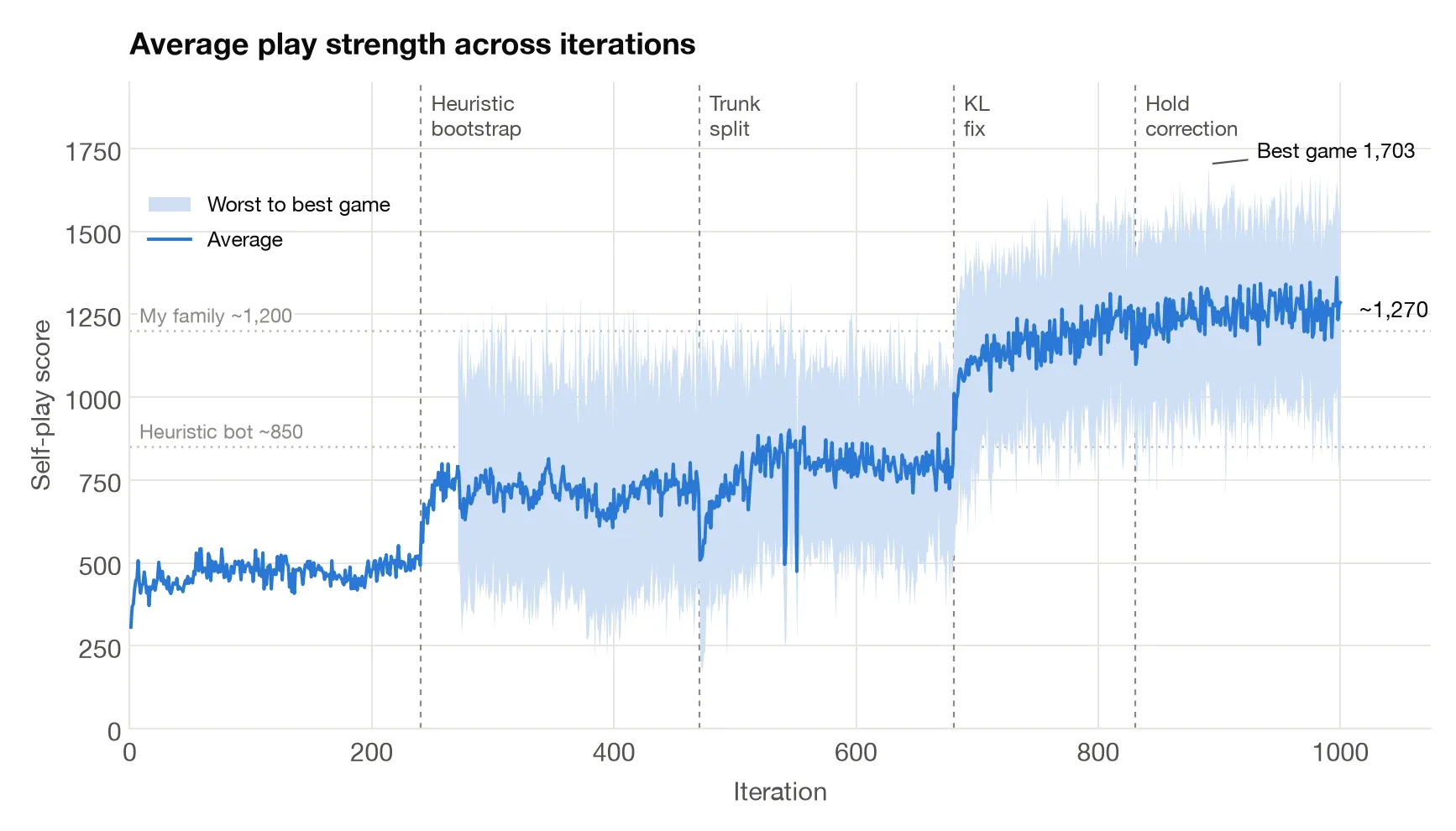
My family averages about 1,200 points a game in Yumbee, which is our version of Yamb, a dice game popular across the Balkans that’s similar to Yahtzee. For scale, random play scores about 230, a simplistic greedy player around 580, and the heuristic bot I built about 850.
After a month and about 1,000 training iterations on my RTX 4090, YoloYamb averages about 1,270 points per game, and you can play against it in the browser. Training took about 390 hours, of which only about 200 were productive, with the rest going to dead-end experiments and various other blunders.
Working With AI
I have a CS background and my job has me working with AI teams every day. So I’m comfortable with the math in ML papers, but I’m not an AI researcher by any stretch. I’ve done scoped ML projects in the past like training a CNN to classify aircraft types and creating an embedding space for music. Going in, I knew training a model with reinforcement learning would be a whole different beast.
Like many previous projects, I wanted to use this project to learn and go deep on understanding the tech. For this reason, early on I decided that every piece of the AI must be built from scratch. Outside of PyTorch and NumPy, YoloYamb uses nothing off the shelf in the model, training, or evaluation workflow. To make this even remotely feasible as a hobby project, I used Claude throughout as my lab assistant. It implemented techniques from the literature, stood up training and evaluation pipelines, helped me work through a bunch of math, and built debug tools that caught many, many mistakes.
On the hardware side, I just used my M1 MacBook Air and eventually my gaming PC, with one RTX 4090 (24GB VRAM) and 64GB of main memory. No clusters or cloud GPUs here! Training typically ran overnight, so when things would crash, I’d find out in the morning and have to restart.
The Approach
The core approach is inspired by AlphaZero from DeepMind. I wasn’t sure if this would translate down to a tiny model trained on a gaming GPU, but I figured it would be fun to try.
The idea is to create a neural network with two heads: a policy head that answers “which action should I take?” and a value head that answers “how many more points is this position worth?” The network plays many games against itself, using search to discover better moves. It then trains on these improved moves and on how the games actually turned out. This makes it better at choosing and evaluating positions, which makes the search stronger the next time around, which then produces better targets to train on, and so on.
Each head has its own loss. Policy loss measures how far the network’s move probabilities are from the search’s improved targets (a cross-entropy), and value loss measures how far its score prediction is from how the game actually ended.
To understand the model, you have to first understand Yamb. Like Yahtzee, you roll five dice, but instead of one column to fill you have several, each with its own rules: one must be filled top-down, another bottom-up, and so on. On top of that, there are bonuses to unlock with careful play, which makes the game less about luck and more about strategy. The best way to get the rules is to try the interactive tutorial or just play a game.
The key challenge with training an AI to play Yamb is that unlike Go or chess, it’s a dice game without any opponent. For example, AlphaZero’s Monte Carlo Tree Search assumes every move leads to a known next position, but with Yamb the dice inject randomness every turn.
So the core search loop for YoloYamb uses expectimax search, which is like classic minimax, but instead of an opponent minimizing your score, you have chance nodes that average over all possible dice outcomes. For each legal move, the search considers every dice roll that could come next, weighted by its probability, and uses the value head to estimate the remaining score of each resulting position.
During training, there are two copies of the network. Each iteration, the raw network trains on a buffer of games for 8 epochs. Those games come from an Exponential Moving Average (EMA) version of the network, which plays 200 games every iteration and adds them to the replay buffer (for a while, some also came from my heuristic bot, which I’ll get to). Using an average network keeps the data stable. To explore, the search mixes 15% random noise into the EMA network’s move probabilities (Dirichlet noise, as in AlphaZero), so it occasionally tries funky moves it would otherwise never learn from. I designed the architecture to play every Yamb variant, but trained only on the modern Yumbee variant to start.
V1: ConvNet Is A Bad Idea (~600 avg)
My first attempt was a 2.94M-parameter dual-head CNN, which I started training on my MacBook Air.
The logic is that a Yamb score sheet is just a 2D grid, like an image. So I fed the 16x8 board into a small convolutional encoder, combined it with the dice and game state, and created two heads: a policy head deciding between all 160 possible moves (128 places to score plus 32 ways to hold dice) and a value head predicting the likely score remaining.
In retrospect, this setup was a pretty terrible idea.
The reason is that convolutions are good at detecting spatial patterns such as “this cell and the one next to it have similar values.” But in Yamb, adjacent columns follow completely different rules. A 3x3 conv filter sliding across three columns at once blurs their identities together, making it super tough for the model to keep these rules straight.
The initial network went from 234 points (basically random) to about 600 in 14 hours of training, learning basics like scoring high dice and not wasting good rolls. But then it plateaued hard, playing barely above a greedy agent (580) and well below the heuristic bot I originally built (about 850).
V2: The Infrastructure Speedup (~600 avg, 10x faster)
Before switching architectures, I got distracted and spent time fixing the training pipeline, which was janky.
V1 played one game at a time, which took forever. Each game has 40+ decisions, each requiring a search then a forward pass on GPU, so the GPU sat mostly idle. To speed up training, I made it so that all 200 games would play in parallel. Every position that needs the network got batched into one combined forward pass, which increased GPU utilization from 1% to 80%.
I then had Claude go to town on optimizations, building tensors directly instead of Python objects, making a Cython port of the encoder and game engine, and creating a more efficient replay buffer. Overall this provided an almost 10x speedup.
It quickly became clear that trying to do this on my old MacBook Air was ridiculous, so I moved training to my gaming PC using WSL, where I’d have access to an RTX 4090.
V3: The Transformer (~720 avg)
Having optimized training, I returned to tackling architecture problems. I tried a few dead-end ideas to tweak the convolutional network until I came upon a realization.
Rather than treating the board as an image, I could treat it as a collection of tokens. By switching to a transformer architecture, perhaps attention could help it better reason between columns and die values during play. This turned out to be the correct metaphor, and it’s the architecture that ultimately powers YoloYamb.
In this architecture, the game state becomes 14 tokens: 8 for the columns, 5 for the dice, and 1 for the game state. These then feed through 6 transformer layers. It’s similar to GPT or BERT except with single-digit millions of parameters, rather than billions or trillions. What’s neat is how naturally attention maps to a game of Yamb. Dice tokens attend to column tokens: “I’m a 6, which columns still need Sixes?” Column tokens attend to dice: “I need 15 more points for the upper bonus, what can these dice give me?”
The heads that ultimately read these tokens took more iteration. My first versions of both the hold head and the value head simply averaged all 14 tokens into one vector. For holds, that was a disaster: averaging mixed five dice with eight column tokens, so the network lost track of which die was which and made obvious blunders. I replaced it with a factored head: instead of scoring all 32 hold patterns directly, each die gets its own keep-or-reroll vote, and the pattern scores are built from those five votes. That fixed the blunders, but independent votes can’t express patterns like straights (1-2-3-4-5), which would come back to bite me later.
Learning everything from random play is slow, so when initial progress stalled around iteration 240, I bootstrapped from my heuristic bot to speed things up. About 30% of training games came from the bot at first, tapering off once the model caught up. Scores jumped right away, and V3 eventually climbed to about 720 on average, peaking at 814, which was promising.
V3.1: The Gradient War (stuck at ~710)
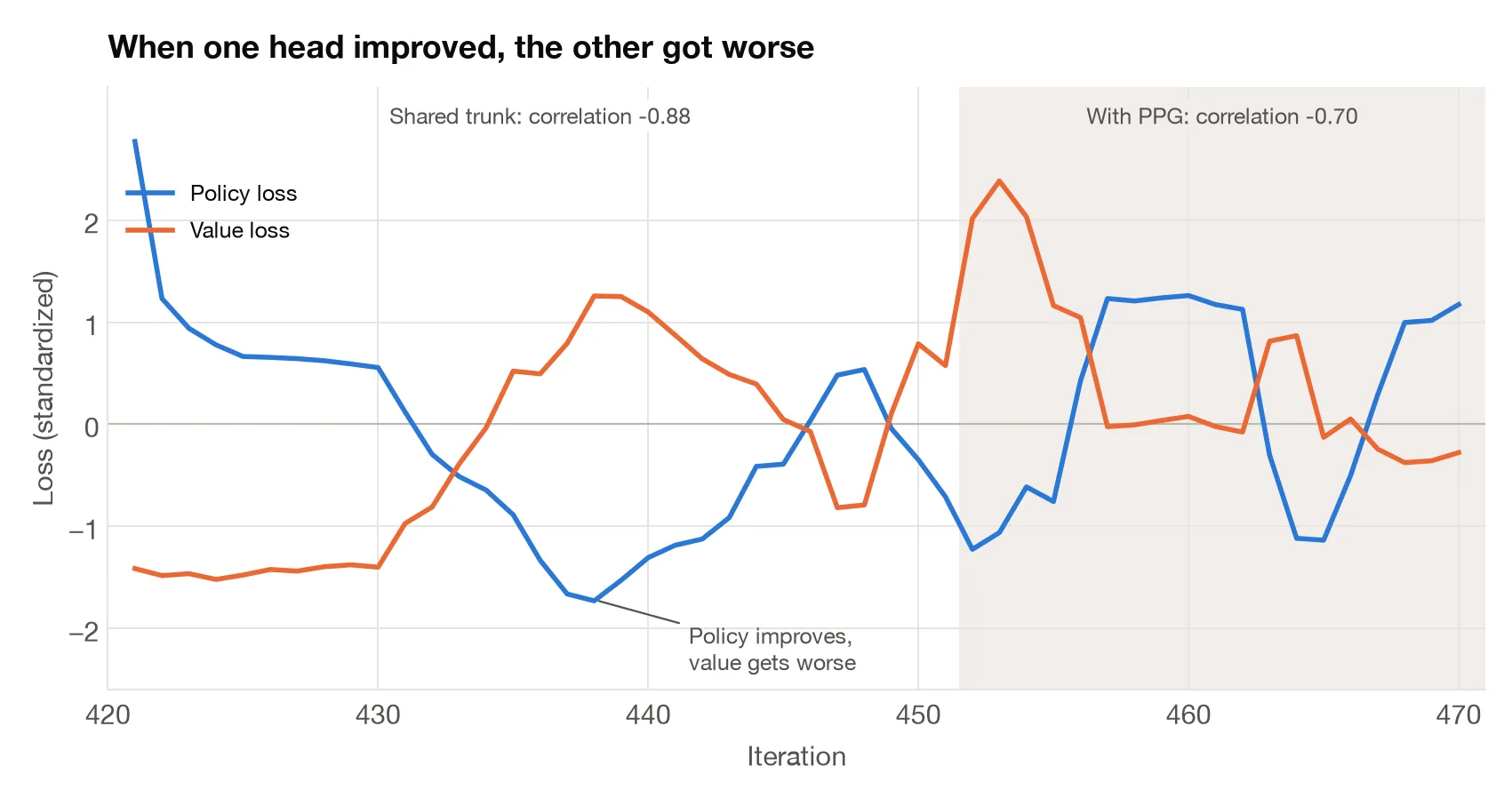
Just as V3 started to pick up steam, scores began swinging 60-80 points every 10 iterations or so. The two heads shared one transformer trunk, and they were fighting over it. When policy loss improved, value loss would get worse, and vice versa.
I initially suspected the value head, which was still averaging tokens. So V3.1’s main change was a better value head that used a learned query to attend over the tokens instead. But as soon as I added it, scores collapsed from 700 to under 300. I blamed the new head and reverted it, but the scores remained collapsed. After much debugging, I found the issue buried in several other changes in the combined resume. Claude had inadvertently changed the code to update the EMA network once per iteration instead of once per batch, which effectively froze the network playing the games. Once I fixed that, I brought the new value head back and scores shot back up. This wouldn’t be the only time subtle bugs crushed progress.
Still battling oscillations, I tried Phasic Policy Gradient (PPG), which targets this kind of issue by alternating which head trains the trunk. Unfortunately it only softened the fight (-0.88 correlation down to -0.70) but didn’t end it. For 100 iterations, nothing improved the average, oscillating around 710. I eventually realized the fix would have to be architectural.
V3.2: Splitting the Trunk (up to ~900, then stuck at ~800)
At iteration 470, I split the trunk so that the first 3 layers stayed shared, but the last 3 were forked into separate policy and value branches. Now neither head’s gradients could majorly fight the other’s. I also further refined the value head to predict a 51-bin distribution of the remaining score instead of a single number, which gave it richer gradients. Scores dropped to 508 after the transplant, then recovered within 10 iterations.
What’s cool is how differently the two branches started to see the dice. When I visualized the die tokens coming out of each branch with UMAP, the policy branch clearly kept each die distinct, since things like “hold die 3” require knowing which die is which. On the other hand, the value branch blended them together, with the five die tokens reaching 0.94 cosine similarity, because value only cares that there are three 6s somewhere.
Probes, Scaffolding, and Crashes
To try and better understand gaps in the model, I had Claude build probes: hand-crafted positions with known-correct answers. One probe showed the network picking Sixes (12 points) over Max (way better with 26 points plus a 63-point bonus) 97.8% of the time. The model was clearly blind to bonuses.
So I gave the model two kinds of help. First, I handed each column token a few bonus features, such as the score gap to triggering the upper bonus, so it didn’t have to work them out from raw scores. Second, I added auxiliary heads that predict bonus progress and the longest straight. The heads don’t tell the network what to do, only what to pay attention to, forcing structural changes in the trunk. For a model this small on a limited compute budget, these were a cheap way to teach it what matters, rather than waiting for it to stumble onto bonuses through millions of self-play games. With this, training took off and hit 900 by iteration 557.
Then I got cocky and stacked six changes into a single restart. The very first iteration exploded, and things kept exploding even after I’d disabled every change. Eventually I discovered I’d interrupted a checkpoint save, and PyTorch happily loaded the half-written file, filling in the missing weights with random values. More checkpoints got corrupted the same way before I made saves fully atomic, and a few other bad changes slowly degraded the network on top of that. Cleaning it all up brought the model back to 834 in one iteration, but not before about 40 hours of GPU time were wasted.
The KL Breakthrough (~800 to 1,000+)
With crashes sorted and training stabilized, the model got back to about 800, but then stalled out again for 100 iterations.
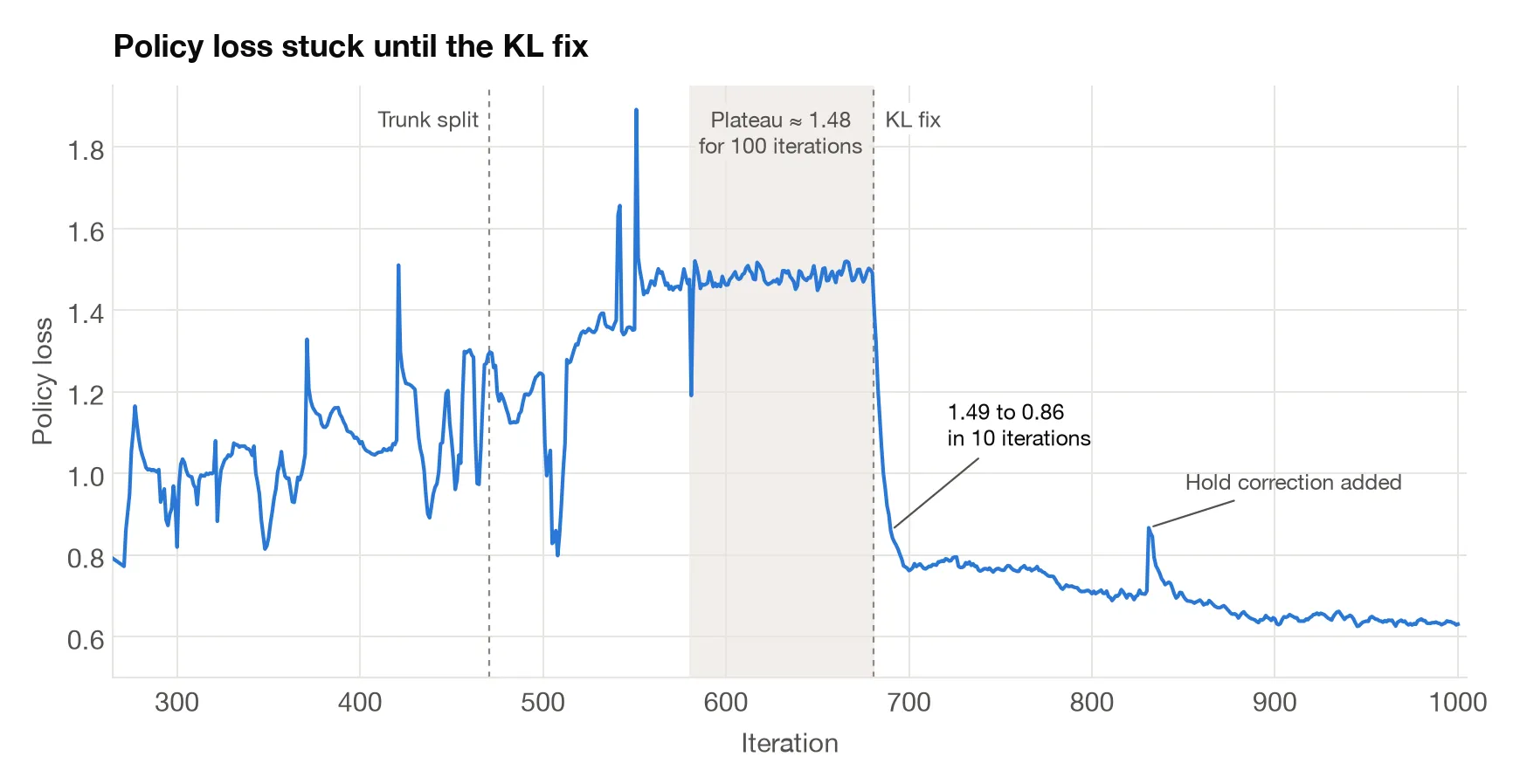
Value loss kept improving from 0.87 to 0.78, which was great. But policy loss was stuck at 1.48, which made no sense. I built various health checks for classic AI problems like exploding gradients, dead neurons, and attention collapse, and spent a lot of time going back and forth with Claude on diagnosis. The eventual culprit was pretty subtle.
To pick a move, the search looks at every legal move and estimates its value, called Q. This value represents the points the move scores immediately, plus what the value head thinks the rest of the game is worth after this move. A softmax turns these into probabilities, so moves with higher Q get more weight and become the training target.
The problem was that the value head’s error in predicting future scores was pretty wide at around 50-100 points. Yet the softmax effectively treated a gap between Q-values above ~8 points as decisive, boosting it above others. It was a noise amplifier!
Luckily, search isn’t the only way to evaluate potential moves. The network’s policy head can also guess how likely each move is to be best. This is the network’s prior. The fix was to combine the network’s prior and the search’s Q-value together:
# Before
target = softmax(Q / temperature)

# After
target = softmax(log(prior) + Q / temperature)
Say you roll five 6s. The policy head is fairly sure scoring those in the Yamb row is best, but the search thinks, wrongly, that scoring in Sixes is 10 points better. Before the fix, the search’s 10-point edge alone decided the target, even though it was just value head noise. The policy kept chasing targets that jumped around, so its loss could never come down. After the fix, the policy’s Yamb prior keeps things anchored. Small, noisy deltas from search only nudge the target, while a move the search finds clearly better still wins. Grill et al. (2020) showed AlphaZero’s search approximates exactly this kind of regularized policy optimization.
Within one iteration, the average jumped from about 800 to over 1,000! I was excited because this was the first time the model started to inch towards expert play, confidently above my heuristic AI. Policy loss also dropped below 1.0 within 6 iterations, a level it had never reached.
V3.3: Home Stretch to Iteration 1000 (~1,270 avg)
The KL fix eventually got V3.2 to about 1,230. At this stage, playing against YoloYamb, it became obvious that it was making weird holds. The per-die hold votes from V3 had finally become the bottleneck. To fix it, I added a correction head that looks at all 5 dice together and can say “hold 1-2-3-4 for the straight.” That broke the ceiling, and two subsequent iterations hit 1,277 and 1,299.
At this point, I noticed that every big jump in scoring followed the same three phases: policy loss drops first, then value loss catches up, and only once both settle do scores spike. It happened with the KL fix, with the hold correction, and once more when I lowered the entropy bonus, a training term that kept the policy from getting overconfident too early. I suspect this behavior is inherent to the shared trunk and split branches, which must “synchronize” somehow to unlock better play and search.
By iteration 1000, the average had settled around 1,270, with a best single game of 1,703. That’s well above my heuristic AI and anyone I’ve played with. How much further it could go was hard to say.
Inside Iteration 1000
Now I’ll walk you through the whole V3.3 network that achieved this. Most of it is a standard transformer, but as you saw earlier, many pieces were bolted on as I learned.
The network works in three stages: a tokenizer turns the game into 14 tokens, a transformer lets them talk to each other, and heads turn them into action.
Tokenizer
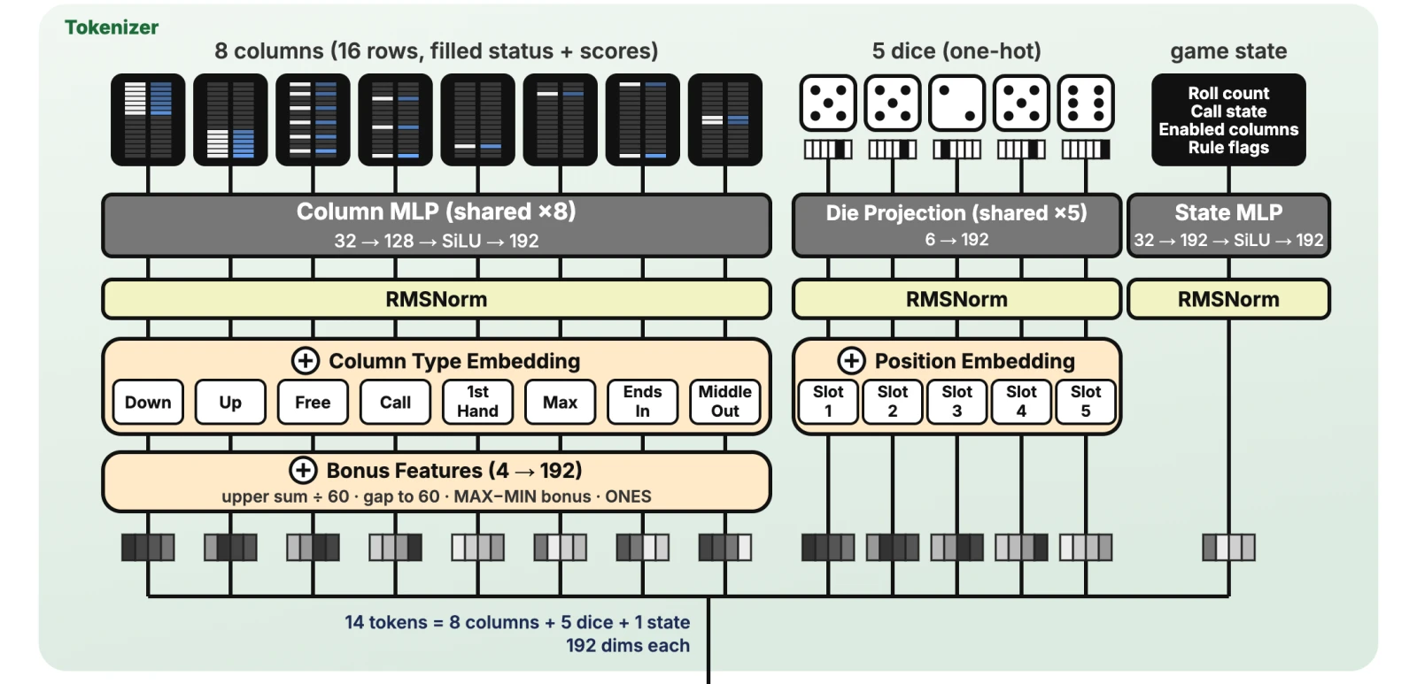
The network has room for 8 columns of 16 rows, enough for every Yamb variant (the Yumbee variant it was trained on uses only 5 columns and 14 rows). Each column token starts as 16 filled/not filled flags and 16 scores (divided by 80 to keep them in a small range). All 8 columns funnel through the same MLP. To ensure they can still distinguish from one another, each column token gets a learned column-type embedding added to it. This is basically the equivalent of a positional embedding in an LLM, but for “which rules apply here” instead of “where am I.” The four bonus features from V3.2 get added on top: the column’s upper-section sum, its gap to the 60-point threshold, its Max-Min bonus, and its Ones count (which multiply that bonus). By iteration 1000, the learned weights on these were about half the size of the column-type embeddings, so the model was clearly using them.
The dice path works similarly. Each die’s face goes through a shared projection, and a slot embedding tells the network which physical die it is, since “hold die 3” needs to know which exact die it is.
The game state token simply summarizes things like roll count, call state, and rule variants. Since iteration 1000 only trained on the Yumbee variant, a bunch of this sat unused.
Transformer
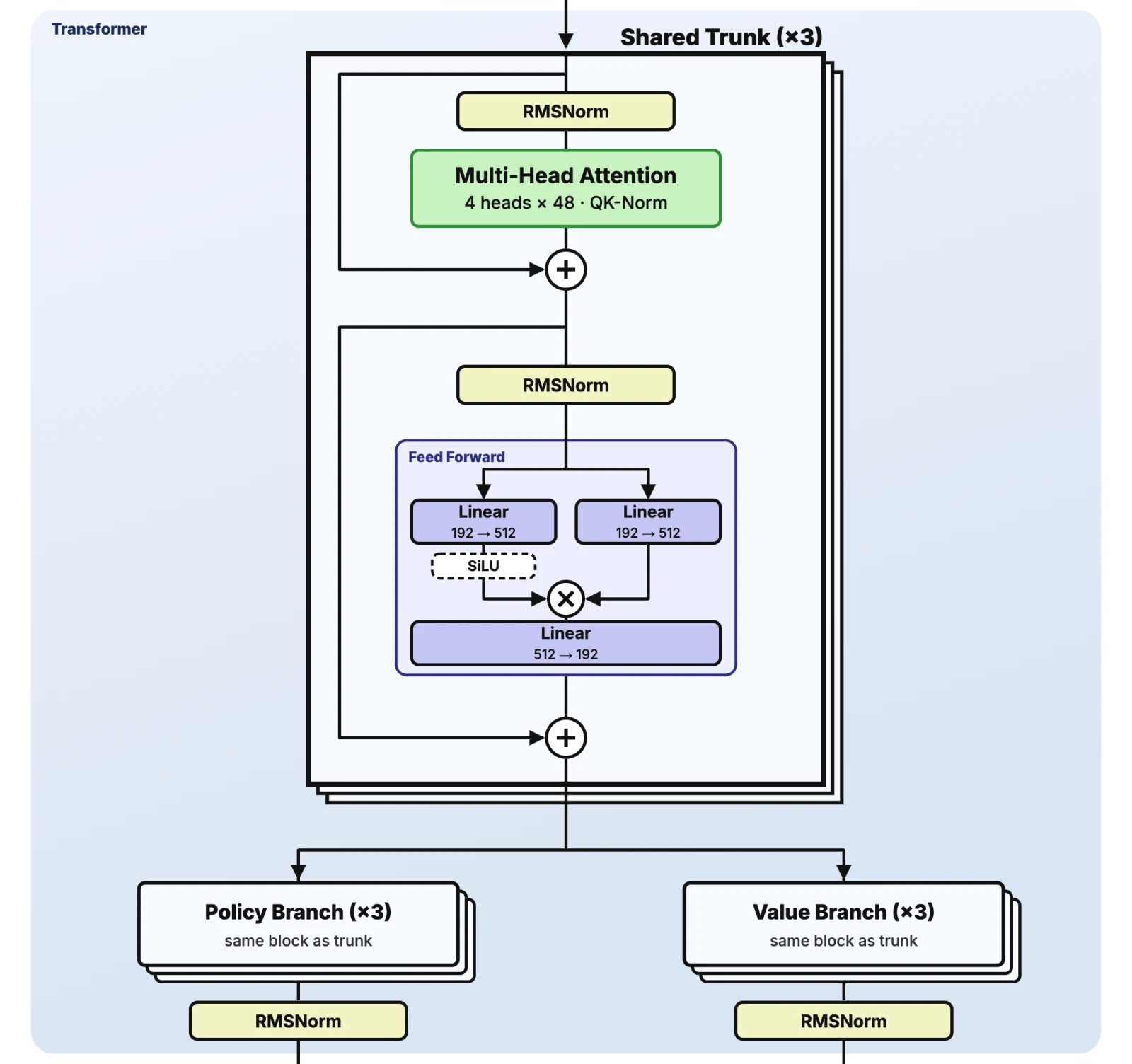
Each transformer block borrows the current best ideas from LLMs: RMSNorm before attention and the feed-forward portion, QK-Norm to keep attention from blowing up, and a SwiGLU feed-forward. The 3 shared layers fork into separate 3-layer policy and value branches, each ending in its own RMSNorm.
I didn’t search for the sizes. When I first built V3, I picked a token width of 192 so the transformer would land at about the same parameter count as V2 (2.96M vs 2.95M), which kept the comparison fair. The feed-forward layer expands each token to 512 dimensions, about 2.67x (8/3) its width, the usual ratio for SwiGLU since it keeps the parameter count of a standard 4x feed-forward. Each layer has 4 attention heads: the 192-dimensional token is split into four 48-dimensional slices (192 ÷ 4), and each head attends using its own slice, so a single layer can follow several relationships between tokens at once without adding parameters. The later bolt-ons, mostly the split branches, grew the network to 4.7M.
Heads
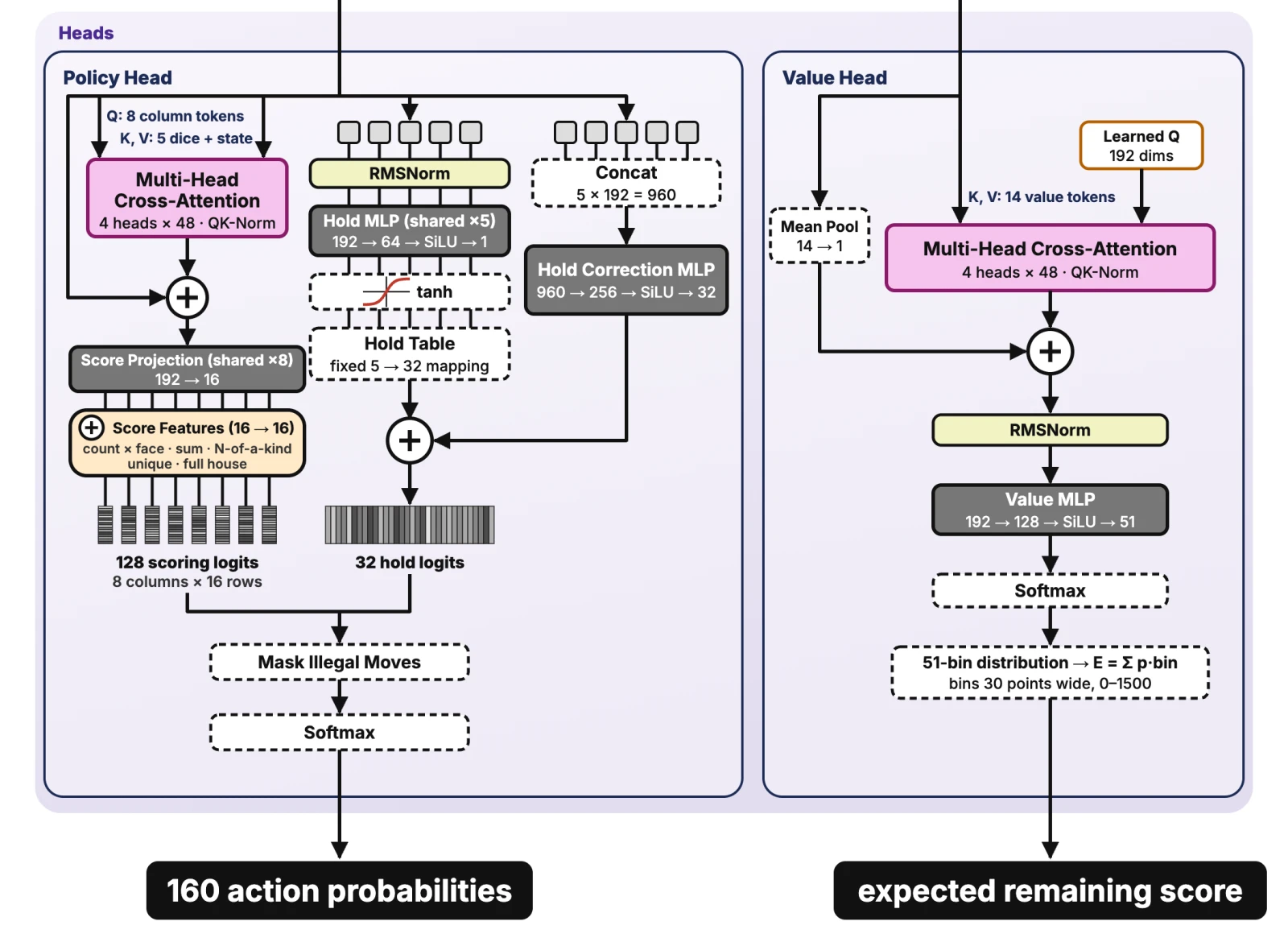
The policy head puts every possible move into one softmax over 160 options: 128 different placements (8 columns x 16 rows) and 32 (2^5) hold patterns for 5 dice, with all illegal moves masked out.
- Scoring: Each column token cross-attends to both the dice and game state, asking “what can I score here with these dice and rules?” Then a shared projection turns that answer into 16 scores per column, one for each row. To save the tiny network from wasting time and capacity learning basic dice arithmetic, score features give the model 16 facts about the dice, like how many 1s, 2s, and so on up to 6s were rolled, their sum, and whether they make a full house, added straight onto those scores.
- Holds: Each die casts a keep-or-reroll vote, squashed by tanh into a -1 to +1 range so no vote dominates. Then, each of the 32 hold patterns scores the sum of its dice’s votes, adding the vote for dice it keeps and subtracting it for dice it rerolls. This way, a die with a strong keep vote boosts every pattern that holds it. The V3.3 hold correction then adds a network-learned adjustment to each pattern.
The value head combines a plain average of the 14 tokens with the learned attention query from V3.1, then a small MLP spreads the prediction over 51 bins, 30 points apart, covering 0 to 1,500. The expected value of that distribution is the network’s estimate of the points still to come.
Conclusions
Building YoloYamb was incredibly difficult and rewarding, and it taught me more about how modern LLMs work than anything else possibly could. A few lessons stuck with me:
- The training loop matters more than the architecture. Once the architecture was roughly right, most of my gains came from fixing subtle bugs in how training worked, like the EMA update and the policy targets, and from making training fast enough to feed the model more data. As Ilya Sutskever once told Dario Amodei, “the models just want to learn.”
- A tiny network and decent compute get you surprisingly far. Iteration 1000 has just 4.7M parameters, a rounding error next to any LLM, and it literally trained on one gaming GPU in about a month.
- You need to measure accurately, especially in a dice game. Two games with the same model can differ by hundreds of points from luck alone, so it was easy to mistake noise for progress and chase ghosts.
Something that’s been continually hard to figure out is what the actual ceiling of Yamb is. With Claude, I estimated it at 1,400-1,500 for the Yumbee variant by measuring how much uncertainty was left in the network’s move choices, splitting it into the part no player could remove (the dice luck) and the part a perfect player would, then converting that gap into points.
My next step is to make the model flexible, since it’s currently only trained on the Yumbee variant for simplicity, even though the architecture supports all variants. But first, I’m convinced the next big jump will come from replacing expectimax with real Monte Carlo Tree Search, the way AlphaZero does it.
Edit (October 2026): A few things I only learned later.
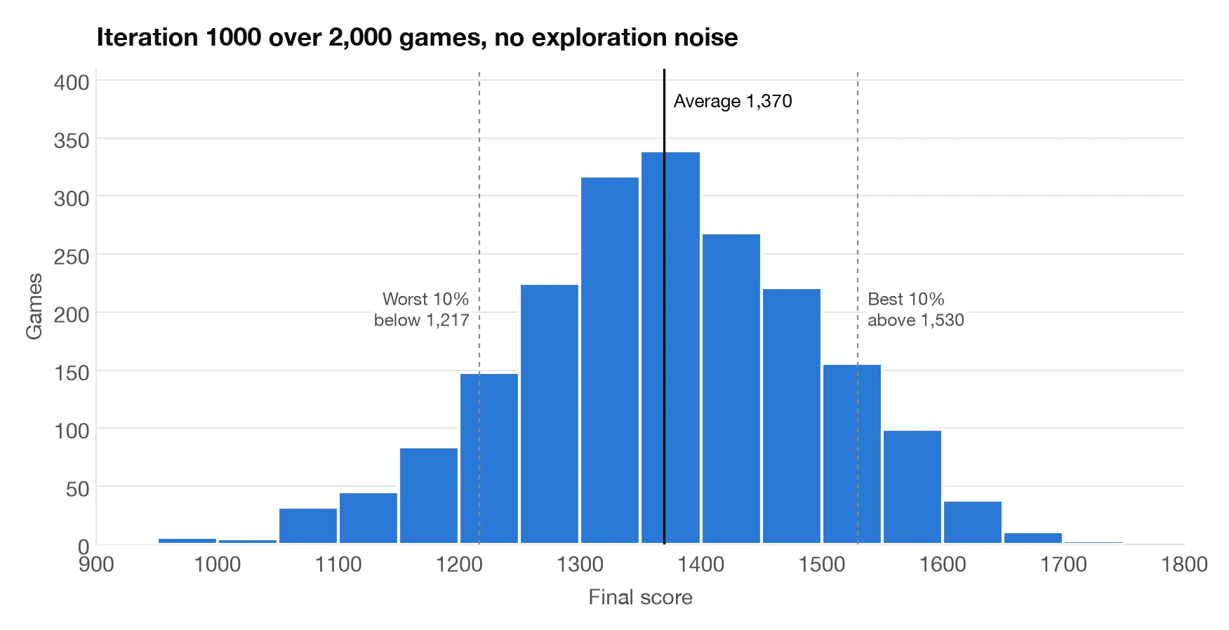
- In retrospect, I made a measurement mistake. Every score above came from training games, which include random exploration noise, and I never properly measured the model with that noise completely removed. When I did, iteration 1000 actually averaged about 1,370 on the Yumbee variant, about 100 points higher.
- My much stronger multi-variant model now averages about 1,470 on the Yumbee variant on the same dice, right in the 1,400-1,500 range I’d estimated as the ceiling of the game. Six months of work only added that much over iteration 1000’s 1,370, so iteration 1000 was already playing much closer to the ceiling than I realized.