Edit (November 2026): I ultimately never went back to MCTS. Later models got all their gains without needing search, and the current one averages about 1,476 on the Yumbee variant playing raw, beating even the clairvoyant search’s 1,383.
One night in July, YoloYamb scored 2,043 points, the first 2,000-point game in the project’s history and what seemed like an absolutely superhuman level of play. My game auditing tool put it at 109% of what optimal play should theoretically score. I deployed it to Yumbee and figured the Monte Carlo Tree Search effort was basically done.
As I’d soon come to painfully realize, none of the gain was real.
The MCTS Plan
YoloYamb is a small neural network I trained from scratch to play Yamb, a Balkan dice game similar to Yahtzee. In my last post, I covered how it got to an average of about 1,270 points a game, well above my family’s 1,200 average (and they’ve been playing for decades). I ended that post convinced the next big jump would come from replacing its search algorithm, expectimax, with Monte Carlo Tree Search (MCTS), the way AlphaZero does it.
Both expectimax and MCTS are different ways of thinking ahead, imagining how the game could play out before committing to a move. My expectimax only looks one move ahead and trusts the network’s value head, its estimate of how many points a position is still worth, for everything after. MCTS looks deeper by running many simulations (imagined playthroughs down the game tree) and spending more of them on moves that keep looking good.
The challenge with using MCTS in Yamb is the dice. In a game like Go, a specific move always leads to the same position. In Yamb, every move is followed by a dice roll, so moves end up with many different results due to luck.
Yamb’s game tree alternates between decisions and chance nodes. Chance nodes are where the search averages over all possible dice rolls, weighted by the probability of hitting different combinations. Rolling all five dice has 252 distinct outcomes; obviously rerolling fewer means far fewer.
After a break to try neural networks for chess (more on that someday), I came back to improving YoloYamb in May and picked up MCTS self-play from the iteration 1000 champion. In self-play, the model plays hundreds of games against itself each iteration, using the search to pick moves, and then learns from the search’s choices. For two months, I experimented with a dozen variants of MCTS, grinding and grinding with nothing moving. Unlike the lead-up to v3.3, during this period the architecture stayed mostly stable, apart from an extra layer added to the end of each branch to improve thinking.
The High
Then in July, everything started to click. I shifted more of the search budget to checking the first roll of each turn and doubled self-play search to 128 simulations.
Soon after, the self-play average jumped from 1,510 to 1,598 in a single iteration, way above the 1,270 score that iteration 1000 had managed in the same kind of games. A few weeks and one lucky overnight run later, the model threw a 2,043-point game. Insane!
To make sure these gains were real, I had Claude build an oracle auditor. It calculated two references. One was a hindsight ceiling score using the actual dice that ended up happening, and the other was an expected-score reference using optimal expected rerolls, bonuses, and column ordering. The latter was meant to estimate what excellent play could score without knowing future rolls, which was a bit more realistic.
The search averaged 1,777 and scored 109% against that expected reference. This wasn’t mathematically impossible, because the reference was an approximation rather than a proven ceiling. At the same time, 1,777 was also about 300 points above the 1,400–1,500 theoretical ceiling I’d estimated previously. That should have made me question the measurements. Instead, I took the audit as confirmation, attributed the discrepancy to the oracle’s limitations, and started to celebrate.
Meanwhile, I had Claude port the search to the browser, so you could play against it on the site (iteration 1000, which was live on the site, didn’t need that). But when I finally went to play this superhuman YoloYamb in the browser, it didn’t feel at all like a 1,777 player. It felt like the original one, maybe even a little worse. Something was off.
You Can See Everything
The browser TypeScript version and Python were supposed to be identical search implementations. My first instinct was that the browser port had bugs causing bad play. So I had Claude start measuring every piece of both implementations.
Unfortunately, it turned out that it was actually Python that had several bugs.
The worst bug was in the chance nodes I mentioned earlier. When the search considers a move, it asks “what happens next?”, which depends on the roll. So the search should try lots of different rolls and average them. To generate those rolls, it reuses the game engine’s own code. To ensure fairness, the engine generates rolls from the game’s seed so that two players in challenge mode, or a player facing off against YoloYamb, see identical dice. Except the search incorrectly reused that same future sequence for all of its playthroughs instead of sampling independent rolls. That meant every time the search asked “what might I roll next?”, it got the actual roll the game was about to make. Instead of averaging over 252 possible outcomes, it saw exactly one, which was the real future one. The search was seeing the dice outcomes before they were rolled.
To make matters worse, holds were subtly broken as well. This is bad because they’re the most important decision in Yamb. After each roll, you pick which dice to keep and reroll the rest. The search got this wrong in two ways:
- Rerolling everything. A flag meant to detect the start of a turn returned true mid-turn, so whenever the search decided what dice to keep, it rerolled all of them, thinking it was just starting. For example, if you have four 6s and roll for the fifth you’ll get a 1-in-6 shot at a big Yamb bonus, but the search priced this move the same as rolling any Yamb from scratch, which is a 1 in 1,300 Hail Mary play.
- Keeping the wrong dice. The network indicates which dice to keep by their position, like “keep the 3rd and 4th die.” But the search applied that to the dice after sorting them, destroying position information. For example, on a roll of 6-1-3-3-5, keeping the 3rd and 4th die would mean keeping two 3s, but in sorted order (1-3-3-5-6) it would mean keeping a 3 and a 5. Totally off.
All this to say, when the search compared holds, it was actually comparing nonsense, and the model was learning its holds from that.
None of these were crashes or showed up in a loss curve. So the bug was super insidious. In fact it all looks great, because search is always finding the best line through clairvoyance.
This all became obvious when I played YoloYamb in the browser. That version of search had its own dice sampling algorithm that correctly drew fresh randomness every time, breaking the clairvoyance.
Subtle Bugs, Unsubtle Collapses
Even with the future peeking fixed, the search was weak. Like so many other bugs I encountered, the reason was again quite subtle.
To keep the GPU busy, MCTS runs 8 simulations at the same time. In a game like Go, that creates a problem. If all 8 simulations pick the same promising move, they walk the same path, reach the same position, and 7 of the runs are duplicated, adding no new information. To solve this, AlphaZero-style searches add a virtual loss, making a move temporarily look worse while one simulation is exploring it, nudging the other simulations to try different lines of play.
Except in Yamb, making the same move doesn’t necessarily cause duplication. You can hit different outcomes because of the inherent uncertainty from dice rolls, trying a wider variety of lines without needing virtual loss. On top of that, when Claude wrote the search, it set the virtual loss to 0.5 as a default, which was way too big and I never questioned it.
To put the 0.5 into perspective, consider that moves are scored on a 0 to 1 scale with a typical move sitting around 0.93. In practice, the difference between the best move and the runner-up is 0.01 or 0.001. A penalty of 0.5 is 50–500 times bigger than that difference! The first simulation took the best move, while the virtual loss forced the remaining 7 onto much worse moves, every single time.
Changing virtual loss on the iteration 1000 model I originally shipped, with eight simulations running in parallel, produced a 1,108 point difference:
virtual loss   score
    0.5          364
    0.0        1,472
It also explained something bizarre I’d been fighting for a while.
The search would only ever compare 8 moves out of about 40, even when I quadrupled the simulation budget. Virtual loss was a big reason, since every batch forced its 8 simulations onto 8 different moves. The other reason was another setting, First Play Urgency (FPU), which gives novel moves a pessimistic starting value so they don’t look unreasonably attractive to search. But, similar to virtual loss, its penalty was 10x bigger than the gap between moves, so once the first batch had selected 8 moves, every other untried move looked decisively worse, so later batches kept revisiting the same 8 moves over and over. Dropping the FPU penalty to zero immediately widened the search to about 18 moves at 64 simulations.
FPU caused another problem too. Since search never tried anything new, exploration noise was effectively gone, and over 90% of search results the model learned from had all their weight on a single move. Yikes.
Back to Basics
With everything sorted, I could finally see what months of MCTS grinding had bought. I measured each model playing raw, with no search helping it.
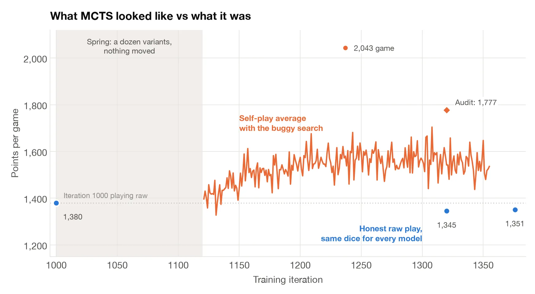
Iteration 1320, the one I’d shipped, played 20 to 35 points worse than iteration 1000. We were going backwards! Double yikes.
A lot of the point loss was because broken search ruined the model’s holding skills. But even non-clairvoyant search, measured over 500 games on the same dice, beat the raw network by just 2.7 points (95% confidence interval: -4 to +9). At 720x the compute cost, the gain was minuscule. My MCTS had been a dud.
But even this measurement was slippery. My first estimate said the unfair peek was worth 279 points, then another different measurement showed only 80 points. When I finally isolated the impact, it turned out the peek changed the chosen move only 1.5% of the time. Clairvoyance had inflated the scores I was looking at, while the hold bugs did hidden damage. I’d stopped trusting the search, and now I couldn’t trust the measurements either.
Measuring For Real
At this point, frustrated, I decided to stop training and fundamentally rebuild how I measure.
From now on, every model would play raw, with no search and no exploration noise, since that’s how it actually plays in Yumbee. Any models being compared would play the exact same seeded dice, reducing the noise from luck. Game counts would be set before a run starts, and every experiment would now include a null arm, an identical copy of the baseline that has to show zero difference.
The result was pretty humbling. Measured raw, iteration 1000 actually averaged 1,370 points, not the weaker 1,270 points I’d measured a few months back. I’d never measured the model without exploration noise, which cost it about 100 points. This also meant MCTS had been trying to improve an already very strong model. The amount of points left to pick up may be very small, well within noise.
With MCTS ruled out, I tried a more tactical route. Hunt for any remaining decisions where the network is provably wrong, verify each fix, and train the model on those fixes.
Each generation had to pass a statistical gate: beat its parent on fresh dice by a pre-determined margin. Four generations in a row successfully passed this gate, accumulating +8.4 points measured over 60,000 games. Small, but it was a lot more trustworthy than the MCTS result.
The Benchmaxxing
With momentum rebuilt, I wanted to find more and more blunders and fix them. But the issue I was running into is that solving Yamb analytically is largely impossible for anything but mostly complete boards. You could find blunders but how would you teach the model to fix them?
I realized that instead of trying to solve a huge board, I could make much simpler versions of Yamb, ones I could solve exactly. With a single column, and Max and Min crossed out to remove the tricky bonus math, a Yamb minigame board has about 250,000 states, low enough to compute fully in a few seconds.
Unfortunately, on those boards, as well as different ones using two columns, the new champion was playing worse than iteration 1000:
gap from perfect play     1 column   2 columns
iteration 1000              44.0       103.0
4 generations later         49.1       109.1
How did this supposedly superior model pass every gate while getting worse at these simpler versions of Yamb? I quickly realized the issue. The gates only checked the average score on full Yumbee games, but the blunders and associated fixes I trained on also came from full games. The model learned to scrape a few more points out of the situations it usually ended up in, while simultaneously losing strength on simpler versions of the same tasks. In other words, the model was benchmaxxed.
Annoyed that I was chasing ghosts again, I almost gave up. But then a different idea hit me. If I could solve small versions of Yamb exactly in seconds, I could also solve hundreds of different ones, and train the model on perfect play examples rather than trying to mine blunders.
And that will be the basis for a future post.